This article is a continuation of a two-part series. For now, we will now discuss our workflow for our document classification project. Firstly, the app's home page automatically pops up when the user executes the main.py file.

As illustrated in figure 1, we present two options. Either the user can run the whole process from training models to predict new coming documents. Or, the user can only use document prediction (based on the specification of a previously trained model).

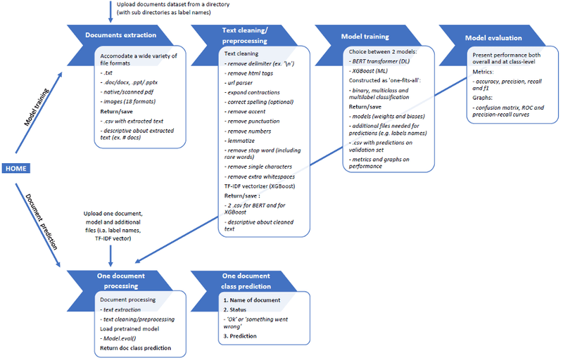
Figure 1. *The overall workflow of the document classification and prediction application*

Python programming for document classification

1. RESTful Flask API

We built two APIs for this project, running concomitantly and for different purposes.

The main API acts as a pivotal framework. It coordinates the whole process and workflow and allowing smooth communication between the user interface and the python objects.

The secondary API is in the main.py file. It retrieves the variables sent to the system when asynchronous requests execute during the navigation through the app (JavaScript). We could not retrieve this information otherwise.

2. Python objects

In total the project counts about ten python class objectsnamong which we present here the most important ones.

The class object 'Extractor' of this file can accommodate a wide number of file formats. This includes native documents files as well as scanned document or images formats. The supported file formats are the following :

document file formats: .txt, .pdf, .doc/.docx, .ppt/.pptx
image/scanned document file format: scanned pdfs, .bmp, .dib, .jpeg, .jpg, .jpe, .jp2, .png, .pbm, .pgm, .ppm, .pxm, .pnm, .pfm, .sr, .ras, .exr, .hdr, .pi

The document extractor relies, amongst other things, on the following libraries: win32com, docx, pptx, pytesseract (OCR), pdfminer, pdf2image;

The class object 'TextCleaner' of this file uses the following NLP text cleaning methods: remove delimiter (e.g. '\n'), remove HTML tags, parse URL (keeping only the domain name such as, for example, ‘cosmetic’ for www.cosmetic.be), expand contraction, correct spelling (optional), remove accent, remove punctuation, remove numbers, lemmatize, remove stop words, remove the single character and remove extra white space.

The correct spelling processing is optional, a user may use it or not use it. For instance, during the navigation through the app interface, see the next section. We recommend using this option only when the text may be of low quality. By this, we mean social media contents with their 'jargonized' language and low-quality scans and/or images where the OCR might produce errors. For text known to be of good quality (e.g., scientific papers or abstracts), it is preferable not to use this option. We noticed that the spell correcting library sometimes replaces correct words with other similar words, e.g. 'physical' for 'topological.'

The 'remove stop word' function is based on a list of stop words constructed during the process. This list is partly based on the existing stop word list provided by some NLP libraries (including sklearn, spacy, gensim, and nltk). This list is also based on the corpus itself, as it includes all the words that only occur in one document. The rationale for including 'rare' words is that they don’t discriminate between classes and may be considered noise.

Besides cleaning the text, TextCleaner also produces the TF-IDF vectorizer needed for running the XGBoost model.

The two models we discussed previously are materialized by two other class objects that have quite the same structure :

Stratified train-validation split
Model training
Model evaluation on the validation set (30% of the total sample)

We needed to accommodate both multiclass and multilabel dataset types during the training. Therefore, we chose to operate a stratified train-validation split instead of the more conventional train-validation split.

When confronted with a multilabel dataset during the training, the model considers the number of original classes and all class combinations presented. Thus, the number of all potential class combinations is much larger than the original number of classes. Some class combinations might have very few documents or even no documents.

Figure 2 presents the value counts of each specific class combination (as multiclass one hot encoded) for a given dataset. As mentioned earlier, we can see that some class combinations do not appear in the count (e.g. [1 0 1 1 1 1]) as they have no document, and some others have very few documents (e.g., class combination [0 0 1 1 0 1] has only one document).

Figure 2. *Value counts of class combinations for a multilabel dataset*

In such a context, the risk with a conventional train-validation split is that some class combinations that the model has not previously seen during the training may be presented during its evaluation. With that respect, the stratified train-validation split ensures that the train-validation split proportion (in our case 70% vs. 30%) is somehow respected within each class combination and that no unseen class combination is presented during model evaluation.

The class object 'Report' offers a detailed and in-depth analysis of the model both overall and at the class level, including, amongst other things, classification reports, confusion matrices, ROC, and Precision-recall curves. Figure 3 shows some examples of outputs from this report.

When the user is satisfied with a model’s performance, the object ‘Prediction’ can predict an incoming unlabeled document class. Before running its code, this object calls the objects ‘Extractor’ and ‘Cleaner’ to preprocess the documents’ text precisely as during the training.

Figure 3. *Examples of outputs from the performance report*

Navigation through the app user interface for document classification

For displaying the HTML files conceived for the user interface, the current project relies on a python-specific graphical user interface (GUI) wrapper (the pywebview package) as it allowed some specific functionalities required for running the code and that would not be permitted with more commonly used web-based GUI (e.g., Google Chrome). During the process, the system needed to retrieve the full path of some files or directories, for example, treating the documents' dataset. While this is perfectly feasible with pywebview, Chrome would upload the file and retrieve the file name (without the path) in similar cases.

We designed the user interface to be self-explanatory and intuitive. Moreover, we tried to give the user control of each step of the process and offer good visibility on how things are running (intermediary reports provided after each step and before launching the next one). The intent here was to help the user to have a good insight into the data, the data processing, and the model quality. Figure 4 shows the home page of the app’s user interface.

Figure 4. *Home page of the app’s user interface*

The document prediction web app

As previously mentioned, the web app only covers the document prediction workflow (and not the model training workflow). In this sense, it uses the same python code as the whole project (but only the classes and functions used for prediction), but some changes must be made regarding the user interface and deployment.

When the user uploads a document, the prediction is automatically processed, and the user is thereafter redirected to the prediction report page, which includes the following output:

The name of the document
Status: 'ok' or 'ko' (meaning that something went wrong: the file format is not supported, or the document is opened in another system/software
Predicted class

Another cge compared to the local app is that the HTML files had to be extracted from pywebview to render them in any web browser/GUI (see Figure 5).

The web app was deployed on Microsoft Azure for testing its proper functioning. We used Docker to create the development environment. For using Docker, two files were created:

The 'Dockerfile' allows us to create a Docker image of the project with all the requirements for running it (including all python packages used by the system).
The file 'docker-compose.yml' gives all the necessary instructions to the hosting environment for launching the app and making it running.

Travis CI is a hosted continuous integration service used to build and test software projects hosted on GitHub. As a complement to Docker, we also used Travis CI to make a direct connection pipeline between the local repository (cloned from the current repository) and the web app deployed on Azure. In the interest of this project, it is easier to update the system with newly trained models.

Conclusion and potential further developments for document classification

Overall, the current project has reached a point where it is well-performing and highly functional (should it be used by inexperienced users or by expert users). As long we present the data to the system correctly (the directory containing the dataset documents with subdirectories as label names), the app can accommodate various file formats and dataset types (for binary, multiclass or multi-label document classification).

In this sense, this project offers highly versatile tools that we can adapt to various business cases. Finally, business applications of the type of the current project are also virtually infinite. To name just a few examples:

Automating the company's documents dispatching (to the right person or the right department);
Automating email dispatching and sorting
Improving the performance of document/text content search engines
Detecting spam or fraudulent/atypical documents
Treating text from medical records to detect pathologies and comorbidities (multilabel-like situation). Although such a system should usefully integrate additional medical data from patients, i.a. medical imagery, test results.

Tech Talk: Document classification and prediction using an integrated application (Part 2)